Simulations

Here we have used “Python” but you may use whatever programming languages that can generate random numbers.

Bernoulli Random Walk

import numpy as np
import matplotlib.pyplot as plt
k = 2000 # number of samples
time_seq = np.arange(0, k)

# Sample a Bernoulli process with p=1/2
X = np.sign( np.random.uniform(-1, 1, k) )

plt.figure(0)
plt.plot(time_seq, X, 'bo')
plt.axis([0, k, -2, 2])
plt.xlabel('Time')
plt.ylabel('X[t]')
plt.grid()
plt.show(block=False)

# ===================================================================
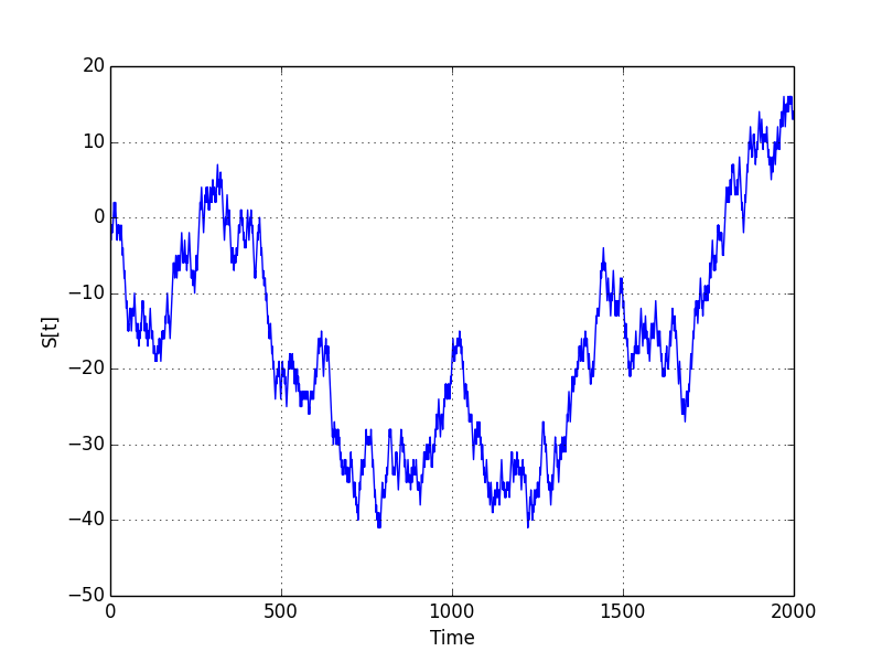
# A random walk based on the Bernoulli process
S = np.zeros(k)
S[0] = X[0]
for itr in np.arange(1, k):
S[itr] = S[itr-1] + X[itr]

plt.figure(1)
plt.plot(time_seq, S)
#plt.axis([0, k, -2, 2])
plt.xlabel('Time')
plt.ylabel('S[t]')
plt.grid()
plt.show(block=False)

# ===================================================================
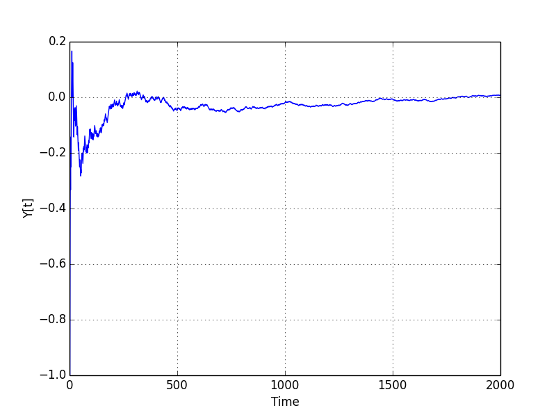
# Y[n] is a normalized version of S[n] by a factor of 1/n
Y = np.zeros(k)
for itr in np.arange(k):
Y[itr] = S[itr] / (itr+1)

plt.figure(2)
plt.plot(time_seq, Y)
#plt.axis([0, k, -2, 2])
plt.xlabel('Time')
plt.ylabel('Y[t]')
plt.grid()
plt.show(block=False)

# ===================================================================
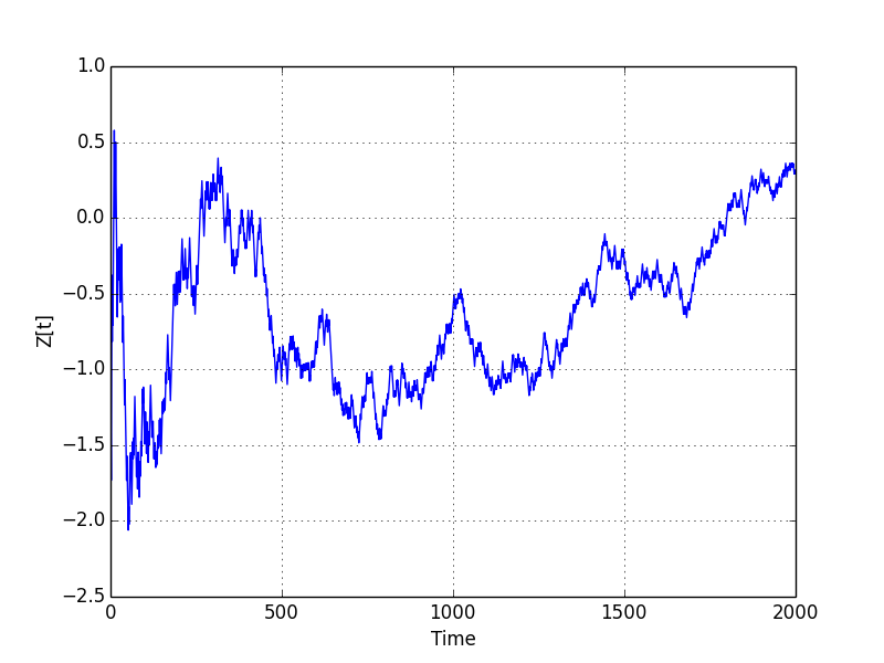
# Z[n] is a normalized version of S[n] by a factor of 1/sqrt(n)
Z = np.zeros(k)
for itr in np.arange(k):
Z[itr] = S[itr] / np.sqrt(itr+1)

plt.figure(3)
plt.plot(time_seq, Z)
#plt.axis([0, k, -2, 2])
plt.xlabel('Time')
plt.ylabel('Z[t]')
plt.grid()
plt.show()

---

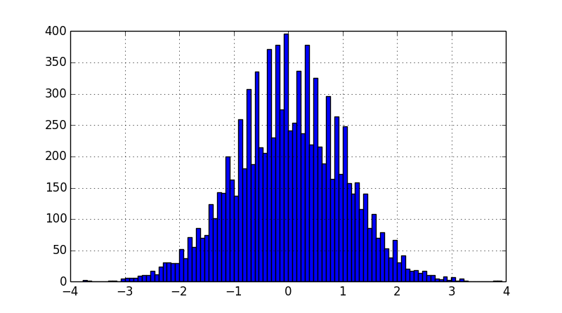
Central Limit Theorem

import numpy as np
import matplotlib.pyplot as plt

N = 10000  # number of independent sample paths
k = 4000  # number of samples in each sample path
time_seq = np.arange(0, k)

# ===================================================================
lst_Z_smpls = np.zeros(N)
for itr in np.arange(N):
    # Sample a Bernoulli process with p=1/2
    X = np.sign( np.random.uniform(-1, 1, k) )

    # A random walk based on the Bernoulli process
    S = np.zeros(k)
    S[0] = X[0]
    for jtr in np.arange(1, k):
        S[jtr] = S[jtr-1] + X[jtr]

    # Z[n] is a normalized version of S[n] by a factor of 1/sqrt(n)
    Z = np.zeros(k)
    for jtr in np.arange(k):
        Z[jtr] = S[jtr] / np.sqrt(jtr+1)

    lst_Z_smpls[itr] = Z[k-1]

plt.figure(0)
plt.hist(lst_Z_smpls, 100)
plt.grid()
plt.show()